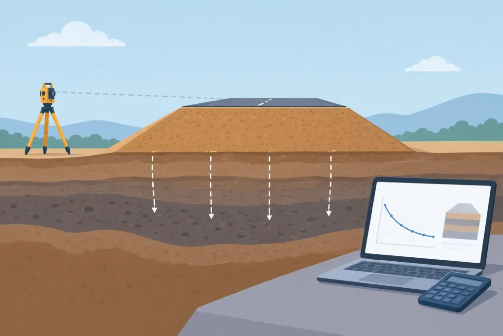
A predicted settlement of 150 mm is not, by itself, a design answer. The critical questions are where it occurs, how quickly it develops, whether it varies along the embankment, and whether the foundation has sufficient stability throughout construction. To calculate embankment settlement reliably, the ground model must be as carefully considered as the calculation method.
For a road or railway embankment on soft clay, most significant movement commonly arises from consolidation of compressible layers under increased effective stress. On granular soils, settlement may be largely immediate. Organic soils, structured clays and fills introduce further uncertainty through creep, disturbance and variable stiffness. A useful calculation separates these mechanisms before combining them into a settlement and time prediction.
Define the ground model before the equations
Settlement calculations are only as defensible as the interpreted soil profile. Start with the embankment geometry, formation level, construction sequence, groundwater conditions and any preloading, vertical drains or ground improvement. Then divide the foundation into layers that have meaning for both stratigraphy and compressibility.
For each layer, establish thickness, unit weight, groundwater level, drainage boundaries and relevant stiffness or consolidation parameters. In fine-grained soils, laboratory oedometer results may provide the compression index, recompression index, preconsolidation stress and coefficient of consolidation. Field data from CPT, piezocones, vane tests and pressuremeters can help identify variability and check whether laboratory specimens represent the in-situ soil.
The distinction between normally consolidated and overconsolidated clay matters greatly. A lightly loaded overconsolidated clay may settle mainly along the recompression line. Once the final effective vertical stress exceeds the preconsolidation stress, virgin compression begins and settlement increases markedly. Treating the full stress increase with a single compression modulus can conceal this change in behaviour.
Calculate embankment settlement from stress increase
The next task is to estimate the vertical stress increment, Δσv, beneath the embankment. For preliminary work, a simplified load distribution may be appropriate. For detailed design, calculate stresses at the centre of each compressible sub-layer using an elastic solution, numerical model or another method suited to the geometry.
An embankment is not an infinite uniform surcharge. Side slopes, widening, variable crest level and nearby excavations all influence the stress bulb. At shallow depth, the stress distribution is particularly sensitive to geometry. In areas where differential settlement is critical, calculate at several transverse and longitudinal positions rather than relying on a single centreline profile.
For a layer represented by a constrained modulus, M, an incremental estimate is:
`Δs = (Δσv / M) × H`
where H is the layer thickness. Divide the layer into sub-layers where stress increment, stiffness or drainage condition changes materially. This approach is practical when a credible modulus has been selected for the stress range concerned, but it should not be used without considering the stress history of clay.
For one-dimensional consolidation, the settlement of a normally consolidated clay layer can be expressed as:
`Sc = H × Cc / (1 + e0) × log10(σ’vf / σ’v0)`
where Cc is the compression index, e0 is the initial void ratio, σ’v0 is the initial effective vertical stress and σ’vf is the final effective vertical stress. If the final stress crosses the preconsolidation stress, calculate recompression to that point with Cr, then virgin compression beyond it with Cc.
The formula is straightforward. Parameter selection is not. Oedometer curves can be affected by sample quality, specimen disturbance and the interpretation of preconsolidation stress. It is generally better to present a central estimate with credible lower and upper cases than to report a precise-looking single value based on uncertain parameters.
Separate immediate, primary and secondary settlement
Total movement is commonly expressed as the sum of immediate settlement, primary consolidation settlement and secondary compression. Keeping these components separate makes the result more useful for construction planning.
Immediate settlement develops as load is applied. In sands and stiff clays it may form a substantial part of total movement. It is commonly estimated from elastic stiffness, adjusted for layer geometry and stress distribution. The selected modulus should reflect strain level, drainage condition and the quality of available field data.
Primary consolidation results from dissipation of excess pore water pressure. In saturated clay beneath a newly placed embankment, loading initially raises pore pressure and reduces effective stress increase. As drainage occurs, effective stresses rise and settlement develops. This is why a long-term settlement estimate alone is insufficient when programme decisions depend on when the settlement occurs.
Secondary settlement, or creep, becomes more relevant in organic soils, peat, very soft clay and materials subject to prolonged loading. A common approximation is:
`Ss = H × Cα / (1 + ep) × log10(t2 / t1)`
where Cα is the secondary compression index and ep is the void ratio at the start of secondary compression. The appropriate start time is judgement-dependent. It should reflect the end of primary consolidation rather than an arbitrary project date.
Predict the rate of consolidation
The degree of consolidation, U, links ultimate primary settlement to settlement at a specified time:
`St = U × Sc`
For a simple one-dimensional layer with known drainage path, U can be obtained from standard consolidation solutions using the time factor:
`Tv = cv × t / Hd²`
Here, cv is the coefficient of consolidation, t is time and Hd is the maximum drainage path. A clay layer draining at both top and bottom has a drainage path of half its thickness. If one boundary is effectively impermeable, the drainage path is the full thickness. This distinction can change predicted consolidation time by a factor of four.
Layered deposits require more care. Permeable seams can shorten drainage paths, while low-permeability crusts or underlying clay can slow drainage. Where vertical drains are proposed, radial drainage, smear effects, drain spacing, discharge capacity and staged loading must be incorporated. A calculation that assumes ideal drain performance can be unconservative in practice.
Account for staged construction and stability
An embankment may be built in lifts because the foundation cannot safely carry the full height at once. Each lift changes stress, pore pressure, strength and settlement. A staged calculation therefore updates the effective stress state at each construction step and allows consolidation between stages.
Settlement and stability are coupled, particularly on soft clay. Rapid loading can generate pore pressures faster than the soil can dissipate them, reducing undrained shear strength and potentially causing failure before the predicted long-term settlement is reached. Check construction-stage stability using appropriate undrained strength data and pore pressure assumptions. The acceptable rate of fill placement should follow from these checks, not merely from the contractor’s programme.
Instrumentation provides the necessary reality check. Settlement plates, extensometers, piezometers and inclinometers can show whether the foundation response agrees with the assumed model. Observational methods work best when trigger levels, actions and decision authority are established before construction. Monitoring without predefined responses is recording, not risk control.
Present results that support engineering decisions
A useful settlement report gives more than a total value. It identifies the adopted soil profile, parameter sources, groundwater assumptions, load stages, drainage conditions and calculation method. It also shows settlement against time, likely residual settlement at handover, and differential settlement over locations that matter to the asset.
For example, a 200 mm total centreline settlement may be manageable if most occurs during a controlled preload period. The same value may be unacceptable at a bridge approach if residual settlement continues after paving or if the transition zone settles unevenly. Geometry, serviceability criteria and construction sequence determine what is tolerable.
Simple, transparent calculation tools are particularly valuable during design reviews and site discussions. On macOS and iOS, Psicons AB develops engineering applications intended to make technical input, calculation checks and result interpretation easy to follow in detail. Whatever software is used, retain the assumptions and intermediate results so that another engineer can review the reasoning.
The best settlement calculation is not the one with the most decimal places. It is the one that states the ground uncertainty clearly, reflects the actual loading sequence and can be tested against field measurements before the embankment becomes difficult to alter.